
PDF CDF and their applications in Machine Learning
Introduction
A majority of aspiring data scientists are either software engineers, freshers or people who do not have a background/degree in statistics. So, sometimes it becomes daunting to keep up with the statistics involved with various Machine Learning techniques.
If you aim to be a good data scientist you need to be on top of your stats game.
With this blog I will try my best to cover these topics:
-
What is PDF?
- Properties of a PDF
- Why do we need PDF?
-
What is CDF?
- Properties of a CDF
- Why do we need CDF?
- Relationship between PDF and CDF
- Where are PDF and CDF used in a machine learning process?
So, lets get to it!
Note: for this blog I am considering that the reader has some prior or minimal knowledge of statistics.
What is Probability Density Function(PDF)?
First let’s take a look at what Wikipedia says:
The PDF is used to specify the probability of the random variable falling within a particular range of values, as opposed to taking on any one value.
Well, thats why I said statistics could be a little daunting. ![]()
Here’s a simpler definition for a Probability Density Function:
Probability Density Function(PDF) of a distribution is basically a smoothed form of its histogram. So, a PDF tells about the frequency of points for a range in the distribution.
In the above definition observe that I mention PDF of a distribution for a range of values and not a single value. The simple reason for that is, finding exact probability of a single value belonging to a distribution will be zero(we will visit this later in this section).
PDF of a distribution can very well be drawn without actual data if type of distribution, mean and variance are known.
Lets take an example to understand this better:
Suppose we plot PDF of ApplicantIncome of 640 people applying for a loan.
Link to data.
# importing required libraries
import pandas as pd
import matplotlib.pyplot as plt
import seaborn as sbn
# Loading data to dataframe
data=pd.read_csv('load_pred.csv')
# plotting PDF of ApplicantIncome
sbn.distplot(data['ApplicantIncome'])
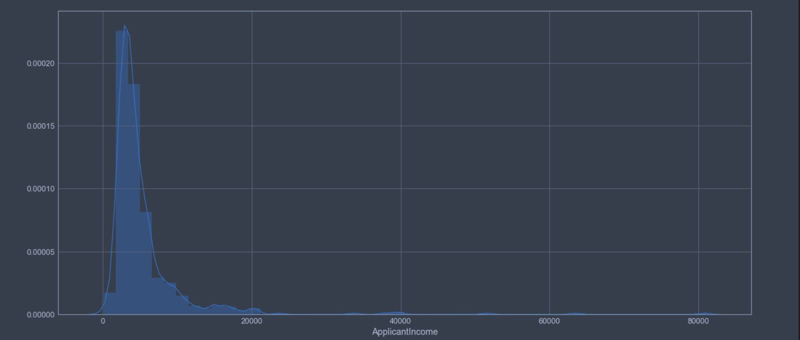
From the above plotted PDF of ApplicantIncome we can see that a majority of points in distribution lie between 0 to 20,000.
Now, our business users ask a question as to approximately what percentage of applicants have an income of <10,000 or how often do applicants with an income of <10,000 apply for a loan?
Since we already have a PDF plotted, all that we need to do now is find the area under the curve <10,000. If you have forgotten how to find the area under curve(AUC), then AUC can be found easily by finding the integral of the PDF over the specified range.
Lets say PDF of our ApplicantIncome distribution(\(X\)) is \(P\):
So, PDF of X can be written as:
\[P(X)\]Hence, area under the curve for \(P(X)\) over the range \(X\in(0,10000)\) will be:
\[\int_{0}^{10000} P(X) dx\]PDF of a distribution over its range is 1. In our example the distribution lies \(X\in(0,80000)\) , hence: \(\int_{0}^{80000} P(X) dx=1\)
Similarly we can find probability of an applicant’s income being \(X\in(10000,20000)\) as:
\[\int_{10000}^{20000} P(X) dx\]Note: Since the probability of a range is given by the integral of PDF curve, the area for probability of a single value will be zero. As the single value will be a line on the X-axis and area of a line=0(line has infinitesimally small width, hence area=0).
Properties of PDF
If \(f(x)\) is a probability density function for a continuous random variable X then:
- \[F(b)=P(X \leq x)=\int_{-\infty}^{x} f(t)dt\]
- \[f(x)\geq0 \text { for any value of } x.\]
- \[\int_{-\infty}^{\infty} f(t)dt=1\]
Lets understand these in plain english:
- First property states that the probability over a range \(X\in(0,x)\) is the integral of the PDF of curve over the region \(0 \text{ to } x\).
- Second property states that PDF of a distribution is non-negative. It makes sense as probability of something happening is always a positive value.
- The third property states that the area between the function and the x-axis must be 1, or that all probabilities must integrate to 1. This again makes sense as the probability of an event to occur cannot be greater than 1.
Why do we need PDF?
As seen above the PDF of a distribution can help us estimate the probability of values belonging to the distribution over a range.
Just by looking at a PDF plot, we can tell the following:
- If the data is normally distributed, about 68% of actual data lies in the range of (\(-1 \times \text {standard deviation}\), \(+1 \times \text {standard deviation}\)). About 95% of data lies in the range of (\(-2 \times \text {standard deviation}\), \(+2 \times \text {standard deviation}\)). About 99.7% of data lies in the range of (\(-3 \times \text {standard deviation}\), \(+3 \times \text {standard deviation}\)). This is also known as the 68–95–99.7 rule.
- Spread of data or variance of distribution.
- Where do majority of the values lie.
What is Cumulative Distribution Function(CDF)?
Lets take a look at Wikipedia’s definition of CDF:
In probability theory and statistics, the cumulative distribution function (CDF) of a real-valued random variable \(X\) , or just distribution function of \(X\) , evaluated at \(x\), is the probability that \(X\) will take a value less than or equal to \(x\).
In simple words:
CDF is the probability that a random variable \(X\)(random variable here is the distribution or data that we are working with), will take a value less than or equal to \(x\). CDF always lies between 0 and 1.
Mathematically:
\[F_X(x)= P(X \leq x )\]This means, for a distribution defined by function \(F(X)\), what is the probability that the points in distribution are less than the value of \(x\).
Properties of CDF
- Every cumulative distribution function \(F(X)\) is non-decreasing.
- Every cumulative distribution function \(F(X)\) is right-continuous.
- \(\lim_{x\to\infty} F_X(x)=1\) , that is CDF for a distribution at positive end of range is 1.
- \(\lim_{x\to-\infty} F_X(x)=0\), that is CDF for a distribution at negative end of range is 0.
Suppose, for the example above we want to find out what is the probability that of all the applicants who apply for loan have an income less than 20000?
Lets plot the CDF for this to answer the question better:
... #Same scaffolding code as above example
# plotting CDF of ApplicantIncome
sbn.distplot(data['ApplicantIncome'],kde_kws={'cumulative': True})
Note that to plot the CDF all we changed in the code was:
# adding kde_kws(Kernel Density Estimation keyword args)
# by specifying cumulative=True we tell seaborn to plot CDF.
 kde_kws={'cumulative': True}
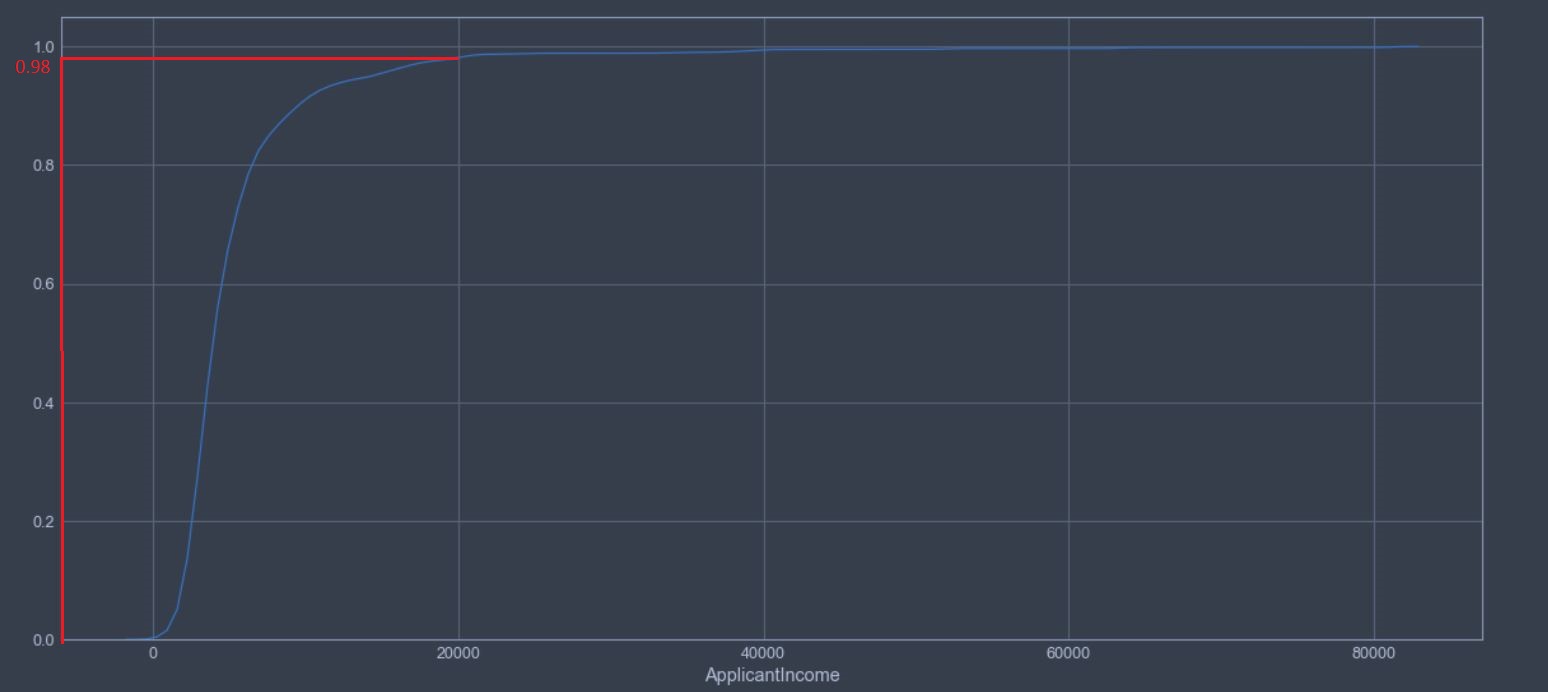
From the above plot we can see that about 98% of applicants will probably have income \(\leq\) 20000.
Why do we need CDF?
By plotting CDF of a distribution we can very easily tell the probability of points lying in distribution \(\leq\) to a given value.
Relationship between PDF and CDF
PDF of a distribution is the differential of its CDF.
Let \(f(x)\) be the CDF for a continuous random variable X. The probability density function (PDF) for X is given by:
\[f(x)= \frac{dF(x)}{dx}\]Similarly CDF of a distribution is the integral of its PDF.
Let \(f(t)\) be the PDF for a continuous random variable X. The cumulative distribution function (CDF) for X is given by:
\[F(X)=\int_{0}^{x} f(t) dt\]Here’s a combined plot of PDF an CDF for ApplicantIncome :
... #same import statements as above examples

# Finding PDF of Applicant Income.
# Note that here I have chosen the number of bins=80,
    # this means that the data will be divided into 80 bins of 1000 each.
# Also I have chosen density=True, so that the function returns probability density values at each bin
    # and normalized such that integral over range is 1.
histogram_vals, bin_vals=np.histogram(data['ApplicantIncome'],bins=80,density=True)
pdf=histogram_vals/(sum(histogram_vals))

# finding cdf.
cdf=np.cumsum(pdf)
#plotting the graphs.
plt.figure(figsize=(20,9)) # setting canvas size
# Plotting PDF of Applicant Income
plt.plot(pdf,label='PDF of Applicant income')
# Plotting CDF of Applicant Income
plt.plot(cdf, label='CDF of Applicant income')
# Setting title of plot
plt.title('PDF & CDF of Applicant Income')
# setting legend for better understanding.
plt.legend(['PDF','CDF'])
# displaying the graphs.
plt.show()
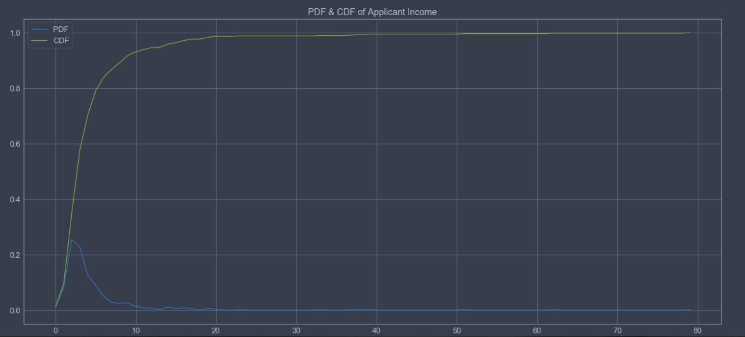
Observations:
- From CDF, the CDF at 2 is 0.1 and CDF at 10 is 0.95. This implies 85% of the data lies in (2000,1000). The percentage of data in any range can be observed from CDF easily in a similar fashion.
- Peak for PDF is at \(\sim 5500\). Hence mean will be at \(\sim 5500\).
It is important to remember that PDF & CDF for a distribution can be drawn or plotted without any actual data if type of distribution, mean and variance are known.
By looking at the PDF we can use the 68-95-99.7 rule to determine the trends in data.
Where are PDF and CDF used in a machine learning process?
PDF and CDF come into picture in the \(2^{nd}\) step of Machine Learning process. In this step we explore the data(this step is known as Exploratory Data analysis(EDA)) at hand and prepare it for consumption by the model.
During Exploratory Data Analysis(EDA) we first do what is called a Univariate analysis(Uni-one Variate- variable*). During univariate analysis we pick one variable and try to understand the trends in data.
* a variable in data science is basically a column of our data, which is independent of other available columns.
During univariate analysis we plot PDF anf CDF of a function to understand the distribution of data and find descriptive statistics like Skewness and Kurtosis.
Lets plot what the PDF will look like corresponding to ApplicantIncome for target variables:
# Setting canvas size
plt.figure(figsize=(20,9))
# finding all rows where Loan_Status = Y
target_0 = data.loc[data['Loan_Status'] == 'Y']
# finding all rows where Loan_Status = N
target_1 = data.loc[data['Loan_Status'] == 'N']
# Plotting PDF of Applicant Income based on the target value.
sns.distplot(target_0[['ApplicantIncome']], hist=False,label='PDF of Applicant income where Loan_Status is Y')
sns.distplot(target_1[['ApplicantIncome']], hist=False,label='PDF of Applicant income where Loan_Status is N')
# Displaying the Graph
plt.show()
Here’s how the graph looks like:
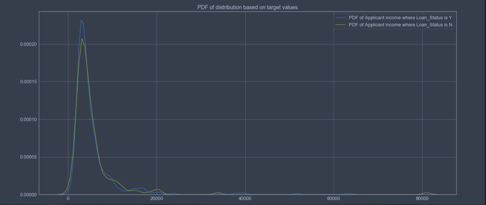
By looking at this graph we can make the following observations:
- Target variable is not linearly separable.
- Most of the values for both the target lie in the region \([0,10000]\)
- There are heavy tails on the right side for both the PDF.
- Heavy tails signify existence of outliers.
- Peak for both the PDF is at \(\sim 5500\). Hence mean for both will be at \(\sim 5500\).
- The distributions are positively skewed. We can apply transformations such as Log transform.
PDF is generally plotted to visualize the distribution of a variable.
PDF can be used to find other descriptive stats like Skewness and Kurtosis. Also, we can easily find mean of distribution just by looking at the data.
CDF tells about what percentage of data lie between what values.
PDF and CDF plots help us to decide what transformations we need to apply to data in order to make it symmetric, linearly separable and find outliers.